

The student, now Ph.D. graduate Viktor Ananiev, was defending a thesis based on work he had done with Alex Read on a statistical issue that arises quite often in data analysis in experimental particle physics: the correct assessment of the statistical significance of an observed feature in the distribution of the data along a variable of interest. Specifically, they developed a method to improve and simplify the calculation of the trials factor in hypothesis testing.
The trials factor is a number that tracks the multiplicity of independent possible places where one could have observed a fluctuation in the data, and is thus used as a multiplier of the estimated probability of a statistical fluctuation.
Suppose, e.g., that I observe that a histogram of my data contains a deviation from the expected behaviour, and I assess that the probability to observe an effect at least as big is one in a thousand. Before I can use that p=0.001 estimate to characterize how significant the observation is, I have to assess how many similar deviations could have potentially arisen in the data I collected. If that number is N, then the global probability that characterizes how significant the effect is can be estimated as N*p. In other words, the trials factor N keeps track of the fact that I did not specify in advance what particular kind of fluctuation I would have been interested in, and suitably "derates" the significance of the phenomenon.
A simple example may be useful to clarify what the whole thing works. Suppose you throw five dice and obtain five sixes: that is a rare and remarkable occurrence. Since the probability to get a six is 1/6, the probability to get five of them out of five is 1/6 to the fifth power, or p=1/7776, which is a rather small number. However, we could argue that the number six does not have more relevance than any other; we would have been equally surprised to throw five ones, or five twos, etcetera. So the trials factor in this case is six - there are six possible equally interesting effects that might arise; a better estimate of the probability of the dice throw is thus 6*1/7776, or 1/1296.
More in general, in physics analysis the trials factor is a concern whenever you are testing a baseline theory of Nature (the bitch, not the journal), which we may call your "null hypothesis". We test it against some alternative scenarios that depend on the value a parameter which does not exist in the baseline theory. Such is the case, e.g., when you search for a new particle whose mass is a priori unknown. You may have produced a histogram of candidate particle mass values, which under the null hypothesis should behave like a smooth and featureless distribution (because those events under the null hypothesis do not contain any special particle, so the mass values are basically random), and be surprised to see that there is an accumulation of events at one particular mass value: is that the signal of a new particle?
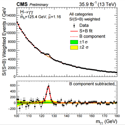
Above, the peak due to Higgs boson production stands on top of a smooth background in this histogram from a CMS search
Indeed, finding systematically the same mass value (or values vithin a short interval, corresponding to the fact that your detector introduces some smearing of the measured mass around the true mass of the particle) is the smoking gun of the existence of a particle. But the same thing could arise because of a statistical fluctuation of the data. A way to estimate the probability of our observation is to fit the data to the null hypothesis and then to the alternative scenario that includes the particle with the mass corresponding to the observed bump: a theorem by Wilks then guides you to taking the likelihood ratio of the two fits, with which you can finally compute the p-value of the effect; however, Wilks' theorem says nothing of the multiplicity of places where a similar fluctuation could have arisen.
Estimating the trials factor by brute force calculation is possible. All you need is to model the distribution that the data should have under the null hypothesis, and then produce a gazillion resamplings of that distribution. Each of the resulting gazillion histograms can be fit, producing a different value of the likelihood ratio. The fraction of times that this ratio is larger than the value you obtained in your real experiment provides the trials factor-corrected probability you want.
The above brute force method is in many cases impractical and very CPU-heavy, and it can be substituted by an approximate calculation first developed by Eilam Gross and Ofer Vitells - two colleagues of Alex Read in the ATLAS collaboration. What Alex and Viktor did was to simplify the Gross and Vitells procedure, and improve the estimate it provides. The work is not trivial and it involves the use of the concept called "Gaussian processes", which we have to space to discuss here today.
The defense
After this long introduction, let me discuss how the PhD defense went yesterday. The two opposers were myself and Prof. Jan Conrad, an astrophysicist from Stockholm University. In other defenses I had attended to as an opposer the discussion was still formal, but not as structured as in Oslo. We had to follow very precise instructions for, e.g., the order with which we were to enter in the auditorium, where we would sit, where we would stand during our questioning of the candidate, etcetera. I was a bit surprised by of course I played along.
What was most surprising to me was the thing I only learned at 8PM the day before the defense: as the first opposer, I would have to give a short introductory lecture to put the research of the candidate in an international, broader context. Needless to say, I spent some late night hours that evening to prepare my talk; but the topic was one on which I had lectured many times in the past, so it was not really challenging to me.
The would-be PhD was thoroughly tortured during the whole day. In the morning he gave a 45 minute lecture in the morning on a topic which was alien from his research area (the title was "Insights in QCD from heavy mesons and baryons"). Then, after lunch the real show begun.
Jan and I had sort of agreed on how to share the kind of questions we would pose to the candidate during our opposition -each of us was expected to spend about 45 minutes for questions, but we could in principle take as much time as we wanted. We were instructed by our Oslo colleagues that we were supposed to be inquisitive and thorough, and really probe the knowledge of the candidate. So we did. In similar situations one of the questioners usually plays the good cop, and the other can be a nastier, bad cop. But in the end we were both rather serious in our questioning. Fortunately, the candidate reacted well. Eventually, after over two hours of discussion, the jury could retreat and then give a positive verdict: a new PhD!
Overall I have to say that the rather formal setup helped make the event more "real" and a true culmination of three years of research for the candidate, so it did work out. As much as the Ph.D. is becoming less important in our society, it is still the highest academic title you can get, and it is the result of fulfilling some necessary obligations that make it worth the effort.
So, congratulations to Dr. Ananiev, and to his supervisor Alex Read. And thanks to Oslo University for having me. Til neste gang!


Comments